Uncertainty in MathHammer using Python
Most existing MathHammer tools (e.g.) will give you, for a given combination of attacker and defender, the expected number of wounds caused or models killed. This is only part of the story though - it’s also useful to look at the distribution of outcomes to get an idea of how likely you are to get that expected value in practice.
The Python code included here is more for reference, and assumes basic familiarity with numpy and pandas.
An Analytic Approach
A typical “expected value” Mathhammer approach will run through code like the shooting_a function below, multiplying out the probabilities to get to the number of models killed.
def shooting_a(bs, s, ap, dmg, t, sv, w, n_shots=1):
    p_miss = (bs - 1) / 6
    p_hit = 1 - p_miss

    if s >= t * 2:
        wound_on = 2
    elif s > t:
        wound_on = 3
    elif s == t:
        wound_on = 4
    elif s <= t / 2:
        wound_on = 6
    else:
        wound_on = 5

    p_not_wound_ = (wound_on - 1) / 6
    p_wound_ = 1 - p_not_wound_
    p_not_wound = p_not_wound_ * p_hit
    p_wound = p_wound_ * p_hit

    sv_ = sv + ap
    p_not_sv_ = (sv_ - 1) / 6
    p_sv_ = 1 - p_not_sv_
    p_not_sv = p_not_sv_ * p_wound
    p_sv = p_sv_ * p_wound

    wounds = dmg * p_not_sv
    models = wounds / w

    ret = pd.Series({
        '# Hit': p_hit,
        '# Miss': p_miss,
        '# Wound': p_wound,
        '# fail to Wound': p_not_wound,
        '# Saved': p_sv,
        '# fail to Save': p_not_sv,
        '# Models Killed': models
    })
    ret *= n_shots
    return ret.to_frame('Expected')
The running example I’ll use in the article is a squard of 10 GEQs firing at an another squad of 10 GEQs. The table below shows what the shooting_a function outputs for this example:
| Expected | |
|---|---|
| # Hit | 5.000 |
| # Miss | 5.000 |
| # Wound | 2.500 |
| # fail to Wound | 2.500 |
| # Saved | 0.833 |
| # fail to Save | 1.667 |
| # Models Killed | 1.667 |
As you can see, this shows the expected number of models killed - but nothing about the distribution.
A Stochastic Approach
It’s possible to work out a mathematical formula that will give you the exact distribution of models killed for a given attacker and defender, but that would be …complicated. It’s much easier to trade off accuracy for mathematical (and computational) simplicity and use a stochastic modelling approach.
The stochastic approach simulates 40k’s shooting mechanics thousands or millions of times (called “iterations” here), each time using random dice rolls. How often each outcome appears (i.e. the number of models were killed on that iteration) gives us the distribution we’re looking for.
Let’s look at the Python code first:
d6is a function that returns the results of rollingndiceshooting_sreturns a table of what happened to each shot (as in our example we have 10 GEQs firing) of each iteration. While the logic looks similar to the analytical codeshooting_a, each line processing a list of thousands of dice rolls rather than a single probability number.
def d6(n):
    return np.random.randint(1, 7, n)

def shooting_s(bs, s, ap, dmg, t, sv, w, n_shots=1, n_iterations=1000):
    n_shots = np.broadcast_to(n_shots, n_iterations)
    n_d6 = n_shots.sum()

    did_hit = d6(n_d6) >= bs

    if s >= t * 2:
        wound_on = 2
    elif s > t:
        wound_on = 3
    elif s == t:
        wound_on = 4
    elif s <= t / 2:
        wound_on = 6
    else:
        wound_on = 5
    did_wound = did_hit & (d6(n_d6) >= wound_on)

    sv_ = sv + ap
    did_save = did_wound & (d6(n_d6) >= sv_)

    wounds = (did_wound & ~did_save) * dmg
    models = wounds / w

    return pd.DataFrame(dict(
        shot=np.arange(n_shots.sum()) - np.repeat(n_shots.cumsum() - n_shots, n_shots),
        run=np.repeat(np.arange(n_iterations), n_shots),
        did_hit=did_hit,
        did_wound=did_wound,
        did_save=did_save,
        wounds=wounds,
        models=models))
The 10 GEQ example
The code to calculate the outcomes for our 10 GEQ example is below; for each of the 1 million iterations it sums the number of models killed by the 10 GEQs, and then for each number of models killed it counts how many times that outcome occurred to work out the probability.
example = shooting_s(4, 3, 0, 1, 3, 5, 1, n_shots=10, n_iterations=1_000_000)
example.groupby('iteration').models.sum().value_counts(normalize=True).sort_index()
This produces the table below. Whereas the analytical approach just said our 10 GEQs would kill 1.667 enemy GEQs, you can see more precisely that there’s a 32% chance of killing 1 enemy GEQ and a 29% chance of killing 2 enemy GEQs. 16% of the time the 10 GEQs won’t kill anything and there’s even a 0.0001% chance they kill 9 of the enemy GEQs!
| # Models | P(Killed = x) |
|---|---|
| 0 | 16.1708% |
| 1 | 32.3604% |
| 2 | 29.0112% |
| 3 | 15.4917% |
| 4 | 5.4128% |
| 5 | 1.3132% |
| 6 | 0.2115% |
| 7 | 0.0261% |
| 8 | 0.0023% |
I mentioned above that this stochastic approach trades accuracy for simplicity, and this table shows two (small) sources of error:
- The expected number of models killed (i.e. the mean) in the example is only 1.665, whereas we know from the analytical approach it’s actually 1.667.
- If an outcome didn’t happen in any of the million iterations then the stochastic approach says the probability is zero. For example, the 10 GEQs didn’t kill 10 enemy GEQs in any iteration so the stochastic approach says there’s an exactly 0% chance of that happening - but in reality it’s possible but very unlikely.
Visualising the Distribution
A useful way of visualing the probabilities of the possible outcomes is a cumulative probability plot, like this:
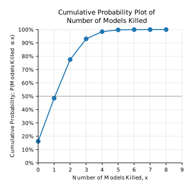
Each point shows the probability of killing at most that number of models. For example, the $x=2$ point shows there’s a 78% chance that the 10 GEQs in the example kill 0, 1 or 2 models. Similarly, the $x=3$ point shows there’s only a 7% chance of the 10 GEQs killing 3 more models.
From the graph you can also see the median value (the first $x$ value that has a $y$ value above 50%) is 2 (compared to the mean of 1.667 and mode of 1) and so the distribution is positively skewed.
Further reading
- A stochastic salvo model for naval surface combat by MJ Armstrong.